Data Analysis

Radial Velocities of a Double-Lined Spectroscopic Binary

I measured how fast each of the two stars in a binary system is moving, using Bayesian statistics and a Monte Carlo sampler.

Year: 2025
Context: Data science course assignment, University of Geneva
Method: Gaussian model fitting, MCMC
Built with: Python, NumPy, SciPy

The physics

The star HD 195521 is actually two stars orbiting each other. We can't see them separately, but their light is recorded together. As they orbit, one moves towards us while the other moves away, and the Doppler effect shifts the light of each star by a different amount.

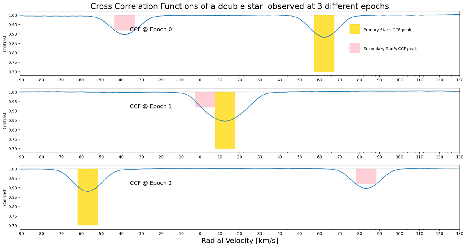
In the data, each star shows up as a dip. The position of the dip gives that star's velocity along our line of sight, its radial velocity. Observed on three different nights, the two dips move apart, merge, and separate again on the other side.

combined light we receive each star's dip, which the model separates

Three panels, one per observation. In the first and third, two separate dips appear at different velocities, on opposite sides. In the middle panel they overlap into a single dip. — The same pair of stars on three nights. Yellow and pink mark my first estimates of where each star's dip is. In the middle observation the two dips overlap.

What I did

Modelled each observation as two Gaussian dips, one per star, and made a first estimate of their positions.
Wrote the log-likelihood of the data given the model, with an extra noise term because the quoted errors were underestimated.
Combined it with priors to get the posterior probability of the parameters.
Sampled the posterior with MCMC, a Monte Carlo method, to get each star's velocity and its uncertainty.
Fitted the three observations together, sharing the shape of each star's dip across nights, which helps most for the overlapping one.

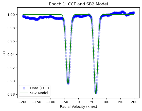
The measured curve with two separate dips, with a green two-Gaussian model following both. — Blue: the data. Green: my two-Gaussian model, before the MCMC fit.

Learning the statistics

The fitting itself was standard data analysis. What made this project useful for me was learning the statistics behind it, such as likelihoods, priors, posteriors and MCMC, and applying them to a real problem instead of a textbook example.

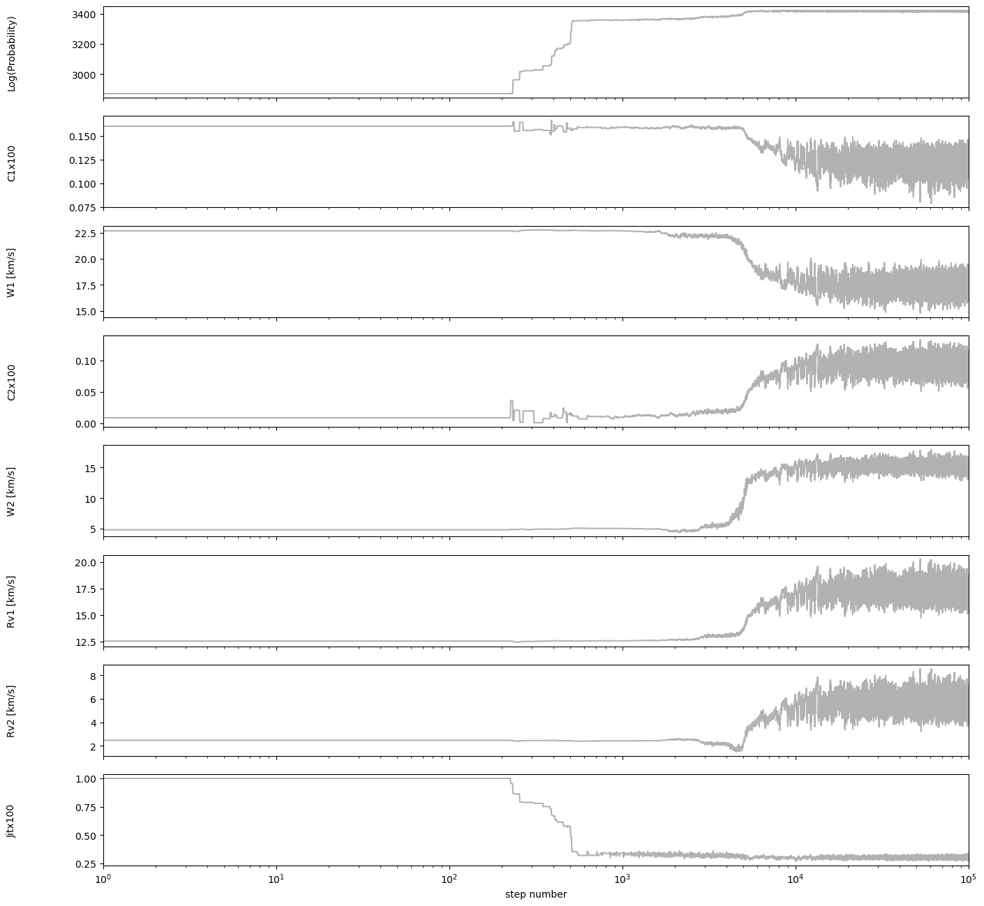
The sampler takes a random walk through the parameters. At first it wanders, then it settles. That first stretch, the burn-in, is thrown away, and the rest gives the result and its uncertainty.

Eight stacked traces, one per parameter, against step number on a logarithmic axis. Each starts flat, shifts, and settles into a noisy band after about ten thousand steps. — The MCMC chains for the overlapping observation. Each parameter shifts at first, then settles into a stable band.

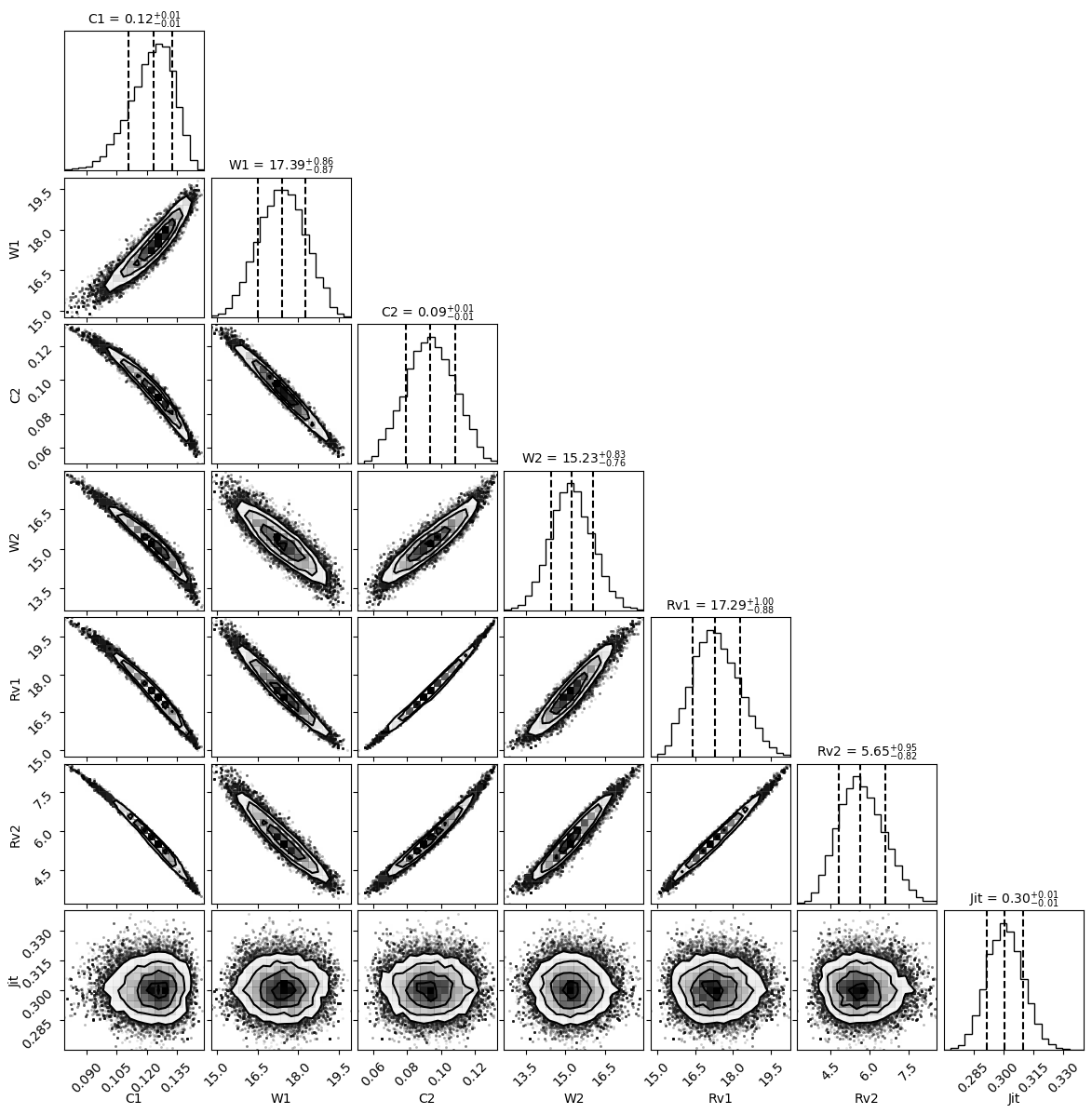
A corner plot of seven parameters. Most pairs form narrow, tilted ellipses, showing strong correlations; only the noise parameter forms round blobs. — For the overlapping observation, almost every parameter is correlated with every other: the model can't fully tell which star is which. Fitting all three nights together reduced this.

What I learned

Writing a likelihood and priors for a real model
Running MCMC and checking it: convergence, burn-in, uncertainties
Reading parameter correlations from corner plots
Fitting models to real astronomical data

Related projects

Convolutional Neural Network from Scratch